CREDIT RISK ANALYZER
1. Introduction:
Context
Banks need to protect their interest before it can take risk on you and issue credit card to you. Banks use their previous credit card holders records for understanding the patterns of the card holders. It is a lot more complex process to predict whether a person who they do not know at personal level, will be a defaulter or not. Banks, along with the data from their own records, also use CIBIL data. Based on all this data, banks want to develop a pattern that will tell them who are likely to be a defaulter and who are not. We have to use this dataset to generate a decision tree model that can successfully predict for a new applicant with recorded data for given parameters in the data set, if he is likely to be a defaulter.Content
The dataset has 13 features with 50636 observations. The features are: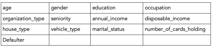
Here age, gender are the age and gender of the card holder.
education is the last acquired educational qualification of the card holder.
occupation can be salaried, or self employed or business etc.
organization_type can be tire 1, 2, 3 etc.
seniority denotes at which career level the card holder is in.
annual_income is the gross annual income of the card holder.
disposable_income is annual income - recurring expenses.
house_type is owned or rented or company provided etc.
vehicle_type is 4-wheeler or two-wheeler or none.
marital_status is of the card holder.
no_card has the information of the number of other credit cards that the card holder already holds.
And at the end of each row, we have a defaulter indicator indicating whether the card holder was a defaulter or not. It is 1 if the card holder was a defaulter, 0 otherwise.
2. Import Libraries:
import pandas as pd
import numpy as np
import seaborn as sns
import matplotlib.pyplot as plt
from sklearn.model_selection import train_test_split, StratifiedKFold
from sklearn.tree import DecisionTreeClassifier
from sklearn.metrics import accuracy_score
from sklearn import metrics
%matplotlib inline
3. Load Dataset:
df = pd.read_csv('credit_data.csv')
4. Data Exploratory Analysis:
df.head()
df.columns
df.shape
df.info()
df.isnull().sum()
df.describe()
df['default'].value_counts()
obj_df = df.select_dtypes(include=['object']).copy()
obj_df.head()
#Looking unique values
print(obj_df.nunique())
print("Gender : ",obj_df.gender.unique())
print("Education : ",obj_df.education.unique())
print("Occupation : ",obj_df.occupation.unique())
print("Organization Type : ",obj_df.organization_type.unique())
print("Seniority : ",obj_df.seniority.unique())
print("House Type : ",obj_df.house_type.unique())
print("Vehicle Type : ",obj_df.vehicle_type.unique())
print("Marital Status : ",obj_df.marital_status.unique())
5. Data Visualization:
def plot_bar_graph(column_name):
    ed_count = column_name.value_counts()
    sns.set(style="darkgrid")
    sns.barplot(ed_count.index, ed_count.values, alpha=0.9)
    plt.title('Frequency Distribution of {} Levels using Bar Plot'.format(column_name.name))
    plt.ylabel('Number of Occurrences', fontsize=12)
    plt.xlabel('{}'.format(column_name.name), fontsize=12)
    plt.show()
def plot_pie_graph(column_name):
    labels = column_name.astype('category').cat.categories.tolist()
    counts = column_name.value_counts()
    sizes = [counts[var_cat] for var_cat in labels]
    fig1, ax1 = plt.subplots()
    ax1.pie(sizes, labels=labels, autopct='%1.1f%%', shadow=True) #autopct is show the % on plot
    ax1.axis('equal')
    plt.title('Frequency Distribution of {} Levels using Pie Chart'.format(column_name.name))
    plt.show()
for col in obj_df.columns:
    plot_bar_graph(obj_df[col])
    plot_pie_graph(obj_df[col])


sns.distplot(df.age, color="r")
plt.show()

sns.distplot(df.annual_income, color="g")
plt.show()

sns.distplot(df.disposable_income, color="b")
plt.show()

6. Data Preprocessing:
Converting Categorical Data to Numerical Data:
def convert_cat_to_num(columns):
    for col in columns:
        df[col] = pd.factorize(df[col])[0]
convert_cat_to_num(df.select_dtypes(include=['object']))
df.head(10)
featurecolumns = df.columns.difference(['default'])
featurecolumns
Checking Data Correlation:
plt.figure(figsize=(14,12))
sns.heatmap(df.corr(),annot=True,fmt="0.2f",cmap="coolwarm")
plt.show()

7. Splitting the Data:
train_X,test_X,train_y,test_y = train_test_split(df[featurecolumns],df['default'], test_size = 0.2, random_state =43)
print (train_X.shape, train_y.shape)
print (test_X.shape, test_y.shape)
8. Model Building and Diagnostics:
1. Decision Tree with Entropy Criterion:
dtree=DecisionTreeClassifier(criterion='entropy',random_state=0
                             ,min_samples_leaf=10
                            ,min_samples_split=10)
dtree.fit(train_X,train_y)
y_pred_entropy=dtree.predict(test_X)
Score_entropy=accuracy_score(test_y,y_pred_entropy)
print("Accuracy: %0.2f" % (round(Score_entropy*100,2)))
cm_dtclass = metrics.confusion_matrix(test_y,y_pred_entropy,labels = [1,0])
cm_dtclass
from sklearn.metrics import roc_curve,auc
def plot_roc_curve(fper, tper):
    plt.plot(fper, tper)
    plt.plot([0, 1], [0, 1], color='darkblue', linestyle='--')
    plt.plot(fper, tper, label='Decision Tree (area = %0.2f)' %auc(fper, tper))
    plt.xlabel('False Positive Rate')
    plt.ylabel('True Positive Rate')
    plt.title('Receiver Operating Characteristic (ROC) Curve')
    plt.legend()
    plt.show()
probs = y_pred_entropy
fper, tper, thresholds = roc_curve(test_y, probs)
plot_roc_curve(fper, tper)

2. Decision Tree with Gini Criterion:
dtree.gini=DecisionTreeClassifier(criterion='gini',random_state=0
                             ,min_samples_leaf=10
                            ,min_samples_split=10)
dtree.gini.fit(train_X,train_y)
y_pred_gini=dtree.gini.predict(test_X)
Score_gini=accuracy_score(test_y,y_pred_gini)
print("Accuracy: %0.2f" % (round(Score_gini*100,2)))
cm_dtclass2 = metrics.confusion_matrix(test_y,y_pred_gini,labels = [1,0])
cm_dtclass2
probs = y_pred_gini
fper, tper, thresholds = roc_curve(test_y, probs)
plot_roc_curve(fper, tper)

9. Cross Validation with Stratified K-Fold:
headers = list(df.columns.values)
x = df[headers[:-1]]
y = df[headers[-1:]].values.ravel()
skf = StratifiedKFold(n_splits=10)
def SKFold(x,y,skf,model):
    dtree_predicted_y = []
    dtree_expected_y = []
    dtree_scores = []

    for train_index, test_index in skf.split(x, y):
        # specific ".loc" syntax for working with dataframes
        x_train, x_test = x.loc[train_index], x.loc[test_index]
        y_train, y_test = y[train_index], y[test_index]

        # create and fit classifier
        model.fit(x_train, y_train)


        # store result from classification
        dtree_predicted_y = model.predict(x_test)

        # store expected result for this specific fold
        dtree_expected_y = y_test

    # save and print accuracy
        accuracy = metrics.accuracy_score(dtree_expected_y, dtree_predicted_y)
        dtree_scores.append(accuracy)
        print("Accuracy for {}: {} ".format(model.criterion,str(accuracy*100)))
        cm_class = metrics.confusion_matrix(dtree_expected_y, dtree_predicted_y,labels = [1,0])
        print(cm_class)
    print("\n")
    print("Max Accuracy for {}: {} ".format(model.criterion,str(np.max(dtree_scores)*100)))
    print("Min Accuracy for {}: {} ".format(model.criterion,str(np.min(dtree_scores)*100)))
    print("Mean Accuracy for {}: {} ".format(model.criterion,str(np.mean(dtree_scores)*100)))
    print("\n")
SKFold(x,y,skf,dtree)
SKFold(x,y,skf,dtree.gini)
10. Results:
Decision Tree with Entropy Criterion: 84.37
Decision Tree with Gini Criterion: 84.24
Decision Tree with Entropy Criterion with Stratified K-Fold: 86.10
Decision Tree with Gini Criterion with Stratified K-Fold: 86.22